Landslide Hazard Proportion
NetMap's Watershed Assessment
Watershed Attribute: The proportion of shallow landslide (or gully erosion) potential as ranked according to five levels of ascending or descending risk. See Shallow Landslide Potential.
Data Type: Grid (raster).
Grids (rasters)
Field Name: LS_GRID
Units: Proportions in 20% increments from highest to lowest
NetMap Level 1 Module/Tool: Mass Wasting/Slope Stability
Model Description
The Shallow Landslide attribute was empirically calibrated to a landslide density attribute (number of landslides per unit area) using landslide inventory data from the Oregon Coast Range. Although specifically targeting topographic, climatic and vegetation conditions in the Oregon Coast Range, the model can be used as a general screening tool in other landscapes. But local empirical calibration is recommended (users creating local calibration is available in NetMap's Tools).
Calculation of shallow landslide potential, in terms of landslide intentisy (density), utilizes a spatially distributed topographic weighting term (see Generic Erosion Potential or GEP) multiplied by a mean landslide density for the region (Miller and Burnett 2007a). The topographic weighting term is determined from locations of landslides mapped in the Oregon Coast Range (Robison et al. 1999). The mean landslide density uses a constant value of 1.0 simply to show intrinsic spatial differences in topographic controls on landslide locations. Topographic weighting ‘w’ is based on the relative density of landslide points found within a specified range of a topographic attribute, such as slope gradient:
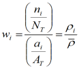
Here wi is the topographic weighting to apply to the ith range of topographic values (e.g., the ith class for values binned into specified classes), ni is the number of landslides mapped within that range of topographic values, NT is the total number of landslides mapped over the study area, ai is the area encompassing that range of topographic values, and AT is the total area of the study site. As indicated, w is a relative landslide density, i.e., the density (rI = ni/ai) of points within a specified range of topographic attribute values divided by the total mean density. The parameter focuses on slope steepness and hillslope curvature or convergence (Figure 1).
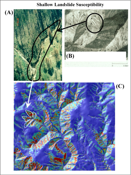
Figure 1. Steep and convergent topography is the target of NetMap’s shallow landslide intensity model. (A) Gully in a post fire landscape in Idaho and shallow failures in bedrock hollows in coastal Oregon (also following a fire).
We calculate a topographic weighting value for every DEM pixel. Multiplied by a specified mean landslide density, it gives a spatially distributed measure of landslide density, in a parameter called ‘Landslide’ (Attribute name = LS_GRID). Integrated over area, or summed over DEM pixels, the relative index of landslide density provides an estimate of how many landslides would be mapped (based on the specified mean landslide density) over any specified area (Figure 2).
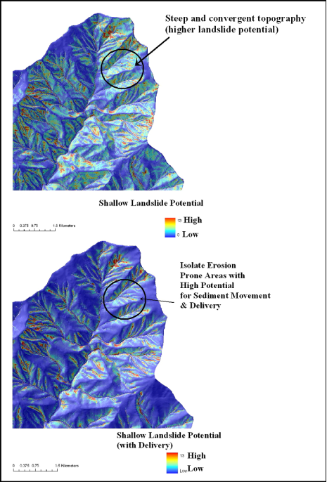
Figure 2. Shallow landslide potential with delivery (bottom) confines those steep and convergent areas most likely to deliver sediment to streams and offers more site specificity for isolating potential erosion areas.
Individual landslide sites in the landslide inventory were geo-spatially referenced on 10-M DEMs and hence the slope gradients associated with failure sites were derived from the DEM (and not from the field measurements) since the goal was to develop a model that utilized a digital database. Consequently, the predicted locations of potential landslide sites (indexed by a variable landslide density) may occur on lower gradient areas (on the DEM), compared to what may be found in the field. In other words, 10-m DEMS commonly underestimate slope gradients. Hence, it is not appropriate to contrast a DEM-based slope gradient map with the predicted landslide density index to compare or contrast slide potential. A slope map can be used as a stand- alone measure of erosion potential, with the understanding that 10-m DEMs underestimate slope gradients. Likewise, the 10-m DEM-based landslide density predictions are a stand-alone representation of shallow failure potential, although the slope gradients associated with failure (on the DEM) are likely less than the gradients that would be measured at those locations in the field.
The model utilized 25-m satellite imagery of forest vegetation (Ohmann and Gregory 2002) that affects landslide density. Younger forests (post clearcut harvest) yield higher landslide rates because of the lower rooting strength compared to mature forests. However, landslide susceptibility in NetMap is predicted using mature forest cover to provide information on the intrinsic potential. Calculations are made at the resolution of the 10-m DEM, which for available USGS-provided data, reflects 40-foot contours mapped at 1:24,000 scale. Because of the empirical calibration, the model is best suited for coastal Oregon, although it should have applications for other mountain landscapes that are prone to shallow failures concentrated in steep and convergent areas. In other areas, the shallow landslide potential parameter is best used as a relative index (high – low).
To get an empirical estimate of landslide-initiation susceptibility, we use landslide density, that is, the number (or area) of landslides per unit land area (e.g., 1.2 landslides per km2, or 536 m2 landslide area per km2). Landslide density is based on the observed number (or area) of mapped landslides. Landslides tend to occur in certain types of locations. For example, translational failure of shallow soil layers – the type of landslide that tends to trigger debris flows in the Pacific Northwest – tend to occur on steep slopes (e.g., Sidle and Ochiai 2006). Such landslides do not occur in low-gradient terrain, and the number of landslides per unit area (landslide density) varies with slope steepness (e.g., hillslopes with gradients between 50% and 60% may have 0.4 landslides per km2, whereas slopes with gradients between 60% and 70% may have 0.8 landslides per km2). One may also look at how landslide density varies with other topographic attributes (contributing area, convergence), and with land cover, soil or rock type, vicinity to a road, rainfall intensity, and so on, but for now we focus on topographic attributes. So to define a spatially distributed estimate of landslide density, we overlay digitized landslide locations on topographic attributes derived from a digital elevation model (DEM).
For example, suppose we have mapped 100 landslides within a 100 km2 watershed, and our DEM-derived slopes show that areas with gradients between 60% and 70% cover 5 km2, and 25 of the mapped landslides lie in those areas. Then those slopes contain 25% of the mapped landslides, cover 5% of the watershed area, and have a landslide density of 4 landslides per km2. Moreover, to assess landslide potential, we assume that in the future, 25% of the landslides that occur in the watershed will, averaged over time, occur on those slopes. We perform the same exercise for every slope class. Each class then has a known landslide density, contains a known proportion of the landslides, and covers a known proportion of the watershed area. The landslide-density calibration for the Oregon Coast Range that we are currently using is shown in Figure 6. Rather than slope gradient alone, we use gradient weighted by a measure of topographic convergence, which for our calibration data better resolves landslide terrain than slope gradient alone (in that a larger proportion of the landslides are included in a smaller proportion of the area). Lacking a better term, we call this quantity a topographic index. Other types of topographic indices may also be defined. In our 2007 paper, for example, Kelly Burnett and I used slope and contributing area, based on the simple model proposed by Montgomery and Dietrich (1994).
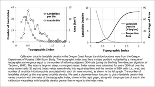
Figure 6. A non linear relationship exists between number of landslides or more specifically landslide density (number/km2, right panel) and the topogrpahic controls of failure (e.g., topographic index). Although the data are from the Oregon Coast Range, the non linear relationship likely holds in many landscapes. This allows the Landslide Intensity parameter to be applied to other landscapes prone to shallow failure, although as a relative index.
Shallow Landslide Intensity-Proportional Risk Assessment
Field Name: LS_PROP_GRID
Another component of the shallow landslide analysis in NetMap, is the ability to represent landslide potential as proportions of risk. Starting with the highest to lowest predicted shallow landslide density, the tool identifies those areas with the highest 20% of predicted landslide risk, then the next highest 20% of risk, and so on. Thus, in Figure 7, the red colors represent those areas with the highest 20% of landslide risk (pixel values), the yellow the next 20% and so on.
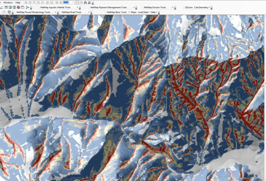
Figure 7. Proportions of landslide risk across a landscape in increments of 20%, starting with the highest 20% (in red). Note that the delivery component (based on a threshold receiving channel gradient) does NOT apply with this attribute. In addition, the mapped distribution of risk categories is sensitive to the area that is examined and the types of topography within it. For example, running the analysis in a small area with very low instability will yield one type of distribution and map, and running it over a larger area with a mix of stability (low to high) will yield another – by default, we are running it at the scale of NetMap datasets (approximately 500,000 acres).
To obtain a value more readily interpreted in terms of relative landslide susceptibility, landslide density is converted to proportion of landslides, area weighted. Using slope-classes, the areas in specific slope steepness-area class are multiplied by landslide density. For example, suppose we have mapped 100 landslides within a 100 km2 watershed, and our DEM-derived slopes show that areas with gradients between 60% and 70% cover 5 km2, and 25 of the mapped landslides lie in those areas. Then those slopes contain 25% of the mapped landslides, cover 5% of the watershed area, and have a landslide density of 4 landslides per km2. Moreover, to assess landslide potential, we assume that in the future, 25% of the landslides that occur in the watershed will, averaged over time, occur on those slopes. We perform the same exercise for every slope class. Each class then has a known landslide density, contains a known proportion of the landslides, and covers a known proportion of the watershed area.
Classes are ordered in terms of decreasing landslide density, the number of landslides in each class (going from least stable – highest density – to most stable – lowest density) are summed to arrive a cumulative total, and then divide by the total to get a proportion. This provides a means to delineate areas in terms of an easily interpreted measure of landslide potential. If we want to delineate the smallest area that includes 25% of all mapped landslides, we’d include all areas with a value greater than zero and less-than-or-equal to 0.25; if we want the smallest area that includes 85% of all landslides, we’d include areas with values greater than zero and less-than-or-equal to 0.85 (Figure 8). The patterns are similar as those shown for landslide density in Figure 7, but in terms of the proportion of (expected) landslides included in any delineated area.
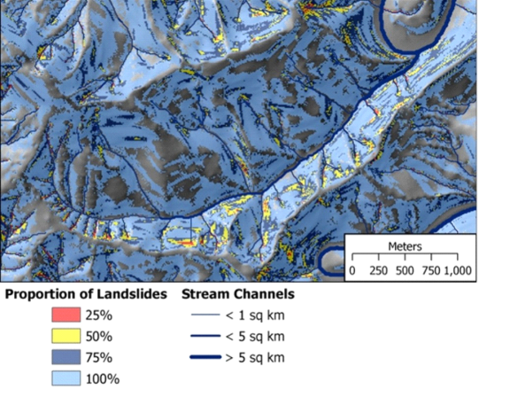
Figure 8. Shown are the areas encompassing a given proportion of expected landslides, starting with the least stable areas (in red). For example red zones cover 25% of the most unstable areas; red plus yellow cover 50% (including 25% of the next highest unstable areas); red, yellow, dark blue and light blue cover all expected landslide terrain. This illustrates the spatially variable nature of hillslope-channel connectivity with respect to mass wasting.
More Background:
There are a variety of models available to predict shallow landslides, primarily for humid mountain landscapes (Sidle 1987, Montgomery and Dietrich 1994, Pack et al. 1998). Most models require information on hillslope topography, including gradients and some measure of convergence. Topographic information provided by 1:24,000 scale mapping does not resolve all topographic features pertinent to landslide locations (Benda and Dunne 1997). For instance, the landslide model does not account for small streamside failures (often referred to as inner gorge landslides) because of the inability of 10-m DEMs to resolve low relief landforms. Mapped landslide potential may also not resolve all small convergent areas, important to project level site-specific assessments. However, mapped landslide potential resolves topographic controls over larger areas, such as the relative risk between different first-order basins or between larger watersheds.
Slope gradient provides a basic topographic index for which relative landslide densities can be calculated. Other options include the SHALSTAB model [Dietrich and Montgomery, 1998] and the product of slope and local drainage area (that within a 10-m radius). For this project, we used the later, because it provided the greatest resolution of mapped landslide locations, in that it requires the smallest proportion of the study-site area to encompass a given proportion of all mapped landslide initiation points (Miller and Burnett 2007a).
The landslide density model allows for a somewhat finer grained resolution of landslide potential (intensity) compared to Generic Erosion Potential (GEP). Although it also focuses on slope gradient and convergence, landslide density values reflect a topographic weighting that is calculated according to a comprehensive shallow landslide inventory. The landslide density predictions (#/km2) pertain specifically to the magnitude of the storm represented in the landslide inventory. For instance, the landslide density is what would be expected during another identical storm. Since there are many storms that can trigger landslides, we recommend that landslide density be used as a relative index (from high to low), although the specific numerical values for landslide density are available in the legend editor and can be displayed if desired. Specific landslide density values to create fixed categories of landslide potential (reflected in the different color codes) can be created to allow comparison across diverse watersheds.
The example mapping of landslide density in the northeastern portion of the Wilson and Trinity River watersheds reveals significant spatial variability. Such maps can be used as a screen by field foresters and geotechnical specialists. Use of generic erosion potential and landslide density predictions can be used to learn how to identify landslide prone areas in the field and from aerial photography.