NetMap's Watershed Assessment
Watershed Attribute: Synthetic Stream Layer
Data Type: Line
NetMap Level 1 Module: Watershed Topography
A digital landscape provides the framework for NetMap's Level 1 Watershed Assessment; typically a 10 m DEM (US National Elevation Dataset [NED]) is used. The digital landscape includes a synthetically derived stream layer produced from a set of flow routing algorithms within NetMap.
The US National Hydrography Dataset (NHD) is often used as a channel mask to guide synthetic channel delineation in low relief and low gradient areas (e.g., all areas less than 4%). Regressions for channel bankfull width and depth are typically obtained from USGS regressions.
NetMap uses several criteria to determine the headward extent of channels within a basin including: 1) critical drainage area (drainage area per unit contour length) or simply drainage area, as a threshold, 2) plan curvature and 3) minimum flow length.
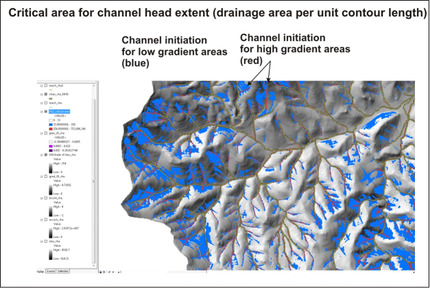
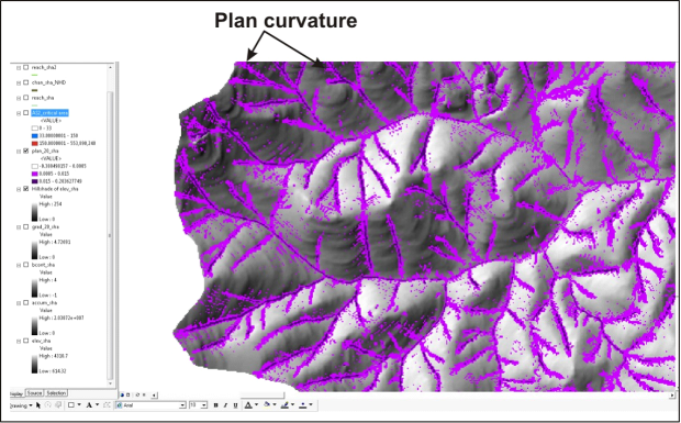
Critical drainage area is drainage area per unit contour length and various thresholds can be used to identify provisional locations of channel heads or channel extent (Figure 1). Critical area is equal to area multiplied by slope gradient-squared (AS2). Threshold values vary with steep and less steep topography, for example, less than 25%, greater than 25% etc. Plan curvature is the curvature of the surface on a cell-by-cell basis, as fitted through that cell and its eight surrounding neighbors. Curvature is the second derivative of the surface, or the slope-of-the-slope. The plan curvature is perpendicular to the direction of the maximum slope (Figure 2). Algorithms for flow direction and channel delineation are described by Clarke et al. 2008.
Figure 1. NetMap’s channel delineation method requires calculating the drainage area per unit contour length, distinct for both steep and low gradient areas. Example is from northern California.
Figure 2. The plan curvature is shown for a basin defined as the second derivative of the surface, or the slope-of-the-slope. The plan curvature is perpendicular to the direction of the maximum slope. The plan curvature is combined with the specific drainage area (Figure 1) and a minimum channel length threshold to define channels and the upward extent of channels. Algorithms for flow direction and channel delineation are described by Clarke et al. 2008.
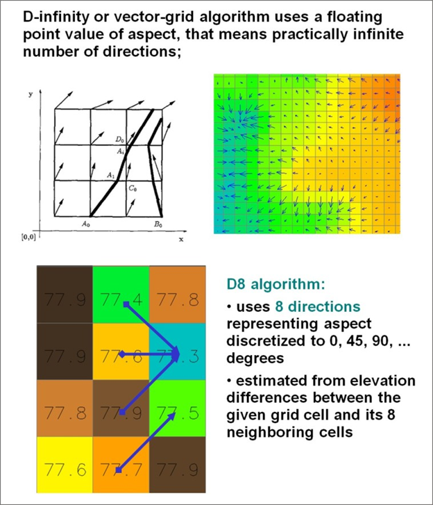
Two flow routing algorithms are used in NetMap. First D-infinity (Figure 3) is used to simulate flow on hillsides (and its convergence) and once a channel head is delineated, the D-8 algorithm is used (Figure 3).
Figure 3. Flow routing on hillsides (unchanneled areas) employs the D-infinity algorithm (top) and flow routing in channels uses the D-8 algorithm (from Mitasova, Geospatial Analysis and Modeling MEA592).
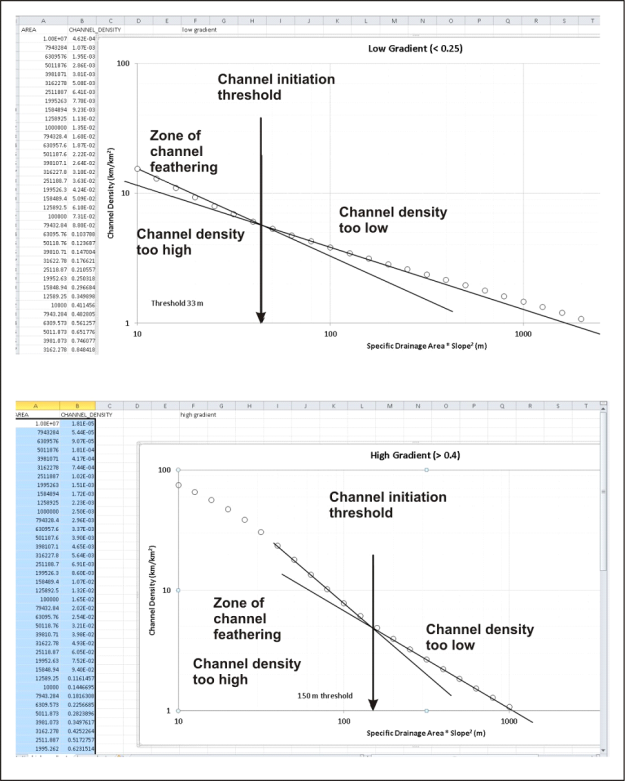
Using both specific drainage area per unit contour length and pan curvature thresholds, a user can manually calibrate the upward extent of channel heads, that is, define the channel density. Too few channels may be created or too many channels. When threshold values are incorrect, there will be “channel feathering” which is manifest as numerous, closely spaced channels extending up on planar hillslopes (Figure 3). The analyst must “calibrate” the thresholds to eliminate or reduce channel feathering (using visual clues of channel locations in landscapes) while providing for a high density of channels. This is done by defining the inflection point between specific drainage area and channel density, given that the threshold for plan curvature is met (Figure 4). The pixel cells that are classified as being a “channel” must extend contiguously for a certain minimum distance, often ranging between 30 to 50 meters, set by the analyst.
Figure 4. Synthetic stream networks derived from DEMs can have too high a drainage density. Here is an example of a synthetic channel network with “channel feathering”, defined as closely spaced channels on planar hillslopes.
Figure 5. To determine the headward extent of the channel network in NetMap requires calculating the relationship between specific drainage area and channel density. There is an inflection point that forms that indicates the transition to an environment of channel feathering (e.g., Figure 3).
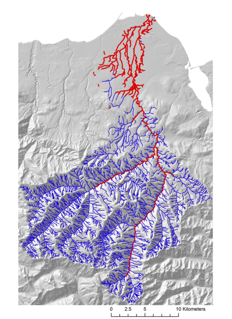
Figure 6. NetMap's synthetic river network showing fish bearing streams (red) and non fish bearing streams (blue).
Typically segment lengths of 50 to 200 meters are used determined by physical properties such as channel gradient, drainage area and width. Thus, many segments are broken at small to large tributary junctions. The network is routed, e.g., each segment “knows” its position in the network, with respect to both upstream and downstream positions. This routed network, allows for information at the channel reach scale to be summarized both upstream and downstream; information can include channel attributes (such as fish habitat potential or road density), hillslope attributes such as erosion potential, vegetation age or fire risk indices), or hillslope information captured by varying buffer widths (see Cumulative Upstream Aggregation and Cumulative Downstream Aggregation for additional information. In addition, channel networks can be trimmed from the top (headwaters) down, These latter functions are available in NetMap's Level 2 Watershed Assessment Tools(by subscription, go here).
NetMap's Level 2 Watershed Assessment Tools(by subscription, go here).
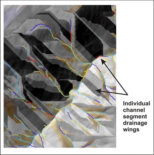
Based on the flow direction grid, “drainage wings” are constructed on both sides of the channel segment thereby delineating the local cumulative drainage area on both sides of the channel (Figure 8). This allows information that is contained in the terrestrial landscape, such as erosion potential, vegetation age, fire risk indices, burn severity rankings (all raster or grid information), and roads to be reported to individual channel segments (Figure 9). This NetMap feature allows unique spatial overlap analyses, such as identifying where the best aquatic habitats are spatially overlapping with the highest risk hillslopes (see Risk Analysis-Overlap tool). Information reported to streams is routed downstream revealing patterns of terrestrial attributes (or channel attributes) at any spatial scale defined by the stream network.
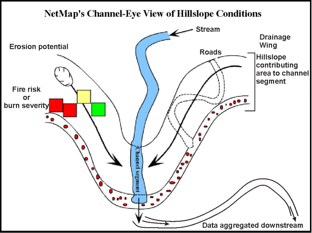
Figure 9. Drainage wings in NetMap allows for information in the terrestrial landscape to be reported to stream channels and then routed downstream, revealing patterns at any spatial scale defined by the channel network.
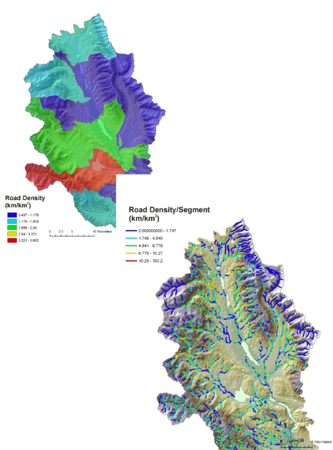
With drainage wings, entire watersheds are discretized into drainage wing facets (Figure 10). Using an average channel length of approximately 100 m, drainage wings average about 0.1 km2 in area. This allows for a finer scale analysis of watershed attributes such as road density (Figure 11).
Figure 10. An example of drainage wings are shown for a basin in California. Using channel segments that average 100 m in length, drainage wing areas are approximately 0.1 km2.
Figure 11. Calculating road density at the stream segment scale provides a much higher resolution mapping of variations in road density. For example, road density in the Clearwater Basin that is calculated at the scale of HUC 6th field subbasins ranged between 0.5 km/km2 and 4 km/km2 (top). In contrast road density measured at the stream segment scale ranged between zero and 100 km/km2 based on the use of drainage wings.